The dbt AI Stack, Upgraded

Graph, Knowledge Graphs, RAG, Reranking, and Full-Text Search, all working together for dbt

Introduction

A few months ago, we published Graph-Powered AI Chat for dbt — and the response genuinely surprised us. The idea of treating a dbt project as a knowledge graph, loading it into FalkorDB, and chatting with it in natural language resonated with a lot of people. We ended up talking about it at the FalkorDB community event and at SQLBits 2026 in Newport, and the conversations there only convinced us there was more to explore.

So we explored.

The original pipeline was already powerful — you could ask complex dependency questions, traverse the graph recursively, and get intelligent answers about your dbt project’s structure. But it had a blind spot: it understood relationships, not meaning. If you asked something like “find models related to revenue reporting,” the graph could only help if you happened to traverse the right edges. It couldn’t understand what a model was about.

That’s what this post fixes.

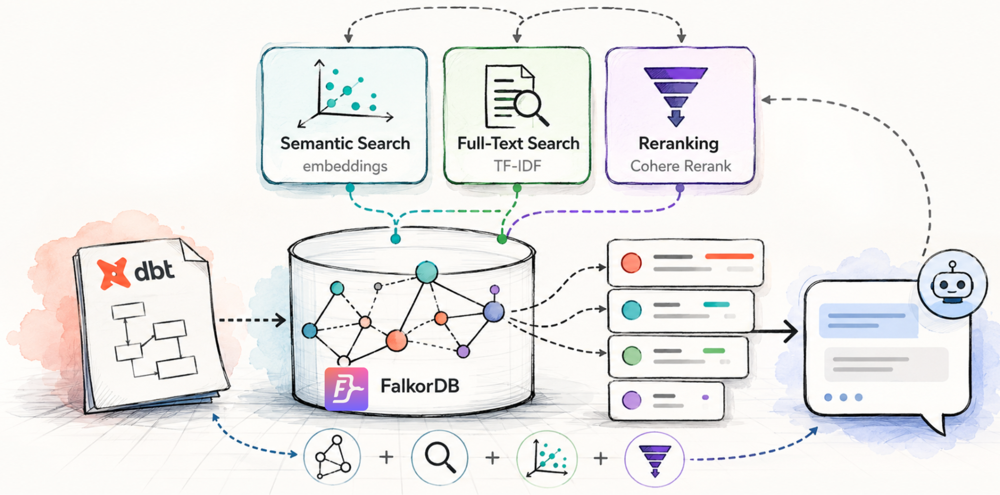
All the changes described here are added to the same repository — dbt-kg — so you can follow along, clone it, and have everything in one place. We’re enhancing the same pipeline with three upgrades that, together, make the system dramatically more capable:

• Semantic search via embeddings — we’ll embed dbt node descriptions directly into FalkorDB, so you can now search by meaning, not just by graph structure. Dependency traversal and semantic similarity, working side by side.

• Full-text search — fast, exact-match keyword search that complements semantic search in ways that matter in practice. We’ll show you why you want both.

• Reranking — once you have multiple retrieval signals, how do you decide what’s actually most relevant? We’ll explain what reranking is, why it matters, and how to wire it in.

By the end, you’ll have a retrieval pipeline that can find what you’re looking for whether you know the exact name, a related concept, or just a vague description. Let’s build it.

Semantic Search via Embeddings

The original pipeline stored your dbt project as a graph — nodes for models, sources, seeds, and snapshots, connected by edges representing dependencies, tests, and macro usage. That structure is fantastic for traversal questions: what depends on what, blast radius analysis, lineage chains. But the nodes themselves were just identifiers. They had no sense of what they meant.

To understand the fix, it helps to understand RAG — Retrieval-Augmented Generation. The core idea is simple: instead of asking an LLM to answer from memory alone, you first retrieve relevant context from your data, then augment the prompt with that context before generating an answer. This is what makes AI systems actually useful on private, domain-specific data — the LLM doesn’t need to have seen your dbt project during training; it just needs the right context handed to it at query time. The retrieval step is usually powered by vector similarity: you embed both your documents and the user’s question into the same vector space, then find the documents whose embeddings are closest to the question.

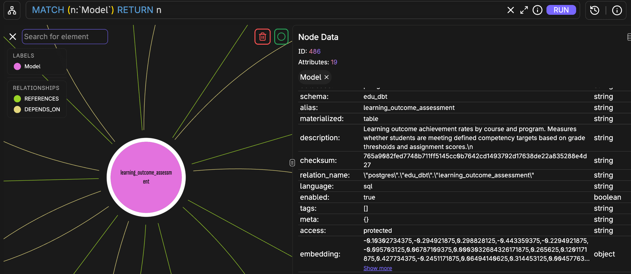
That’s exactly what we’ve added here. For each node, we take everything meaningful about it — its name, resource type, schema, materialization, description, and all its column descriptions — concatenate it into a single piece of text, embed it, and store that embedding directly as an attribute on the node in FalkorDB. No separate vector store, no extra nodes, no parallel data structure to keep in sync. The embedding lives on the same node as everything else.

This happens automatically when you upload your manifest.json and catalog.json — the upload endpoint calls build_node_embeddings() right after the graph is loaded, so by the time you open the chat, every node is already searchable by meaning.

At query time, the FalkorDBNodeRetriever takes your question, embeds it using the same model, and runs a KNN vector search across all node labels simultaneously. The results are ranked by cosine similarity — no Cypher required, no need to know any model names upfront.

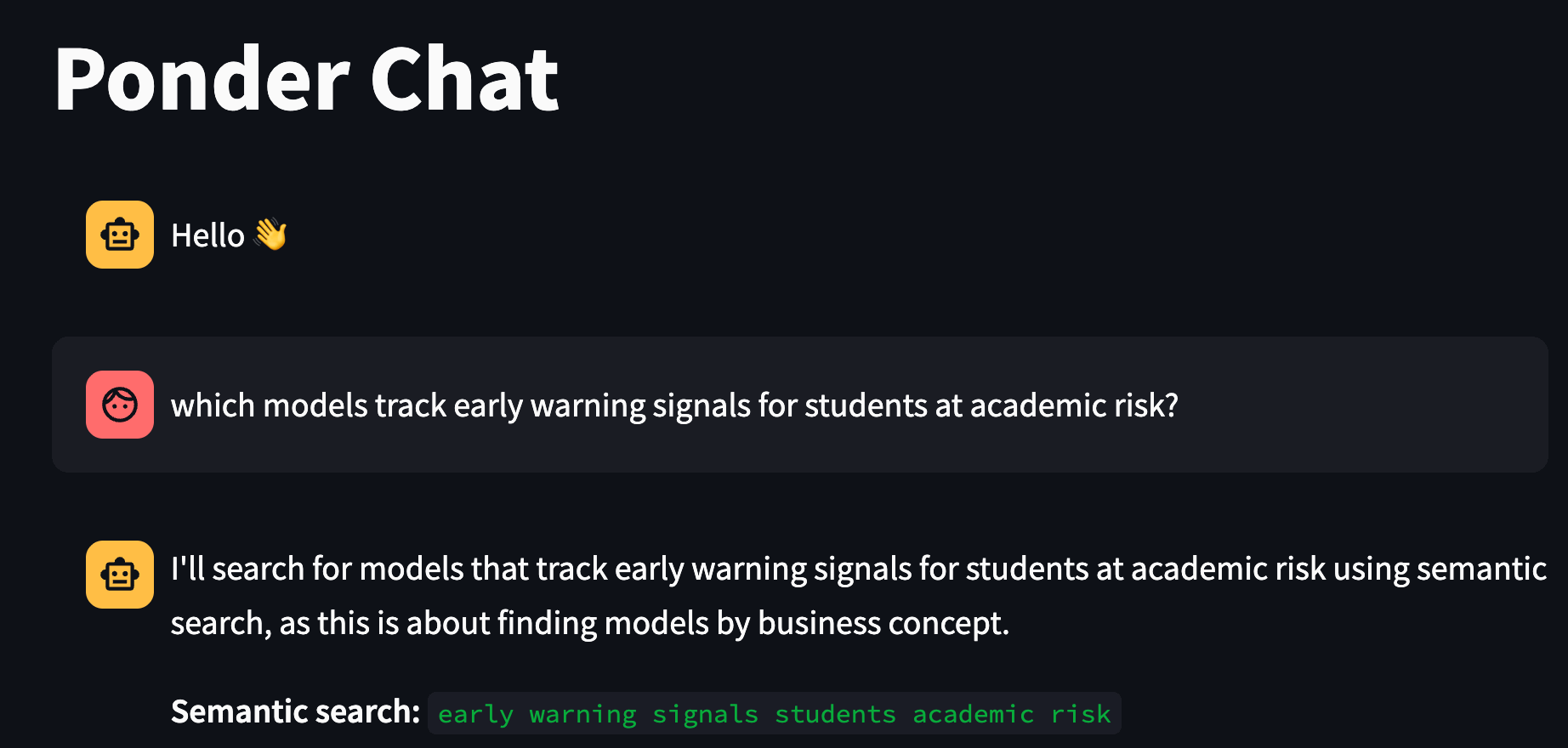
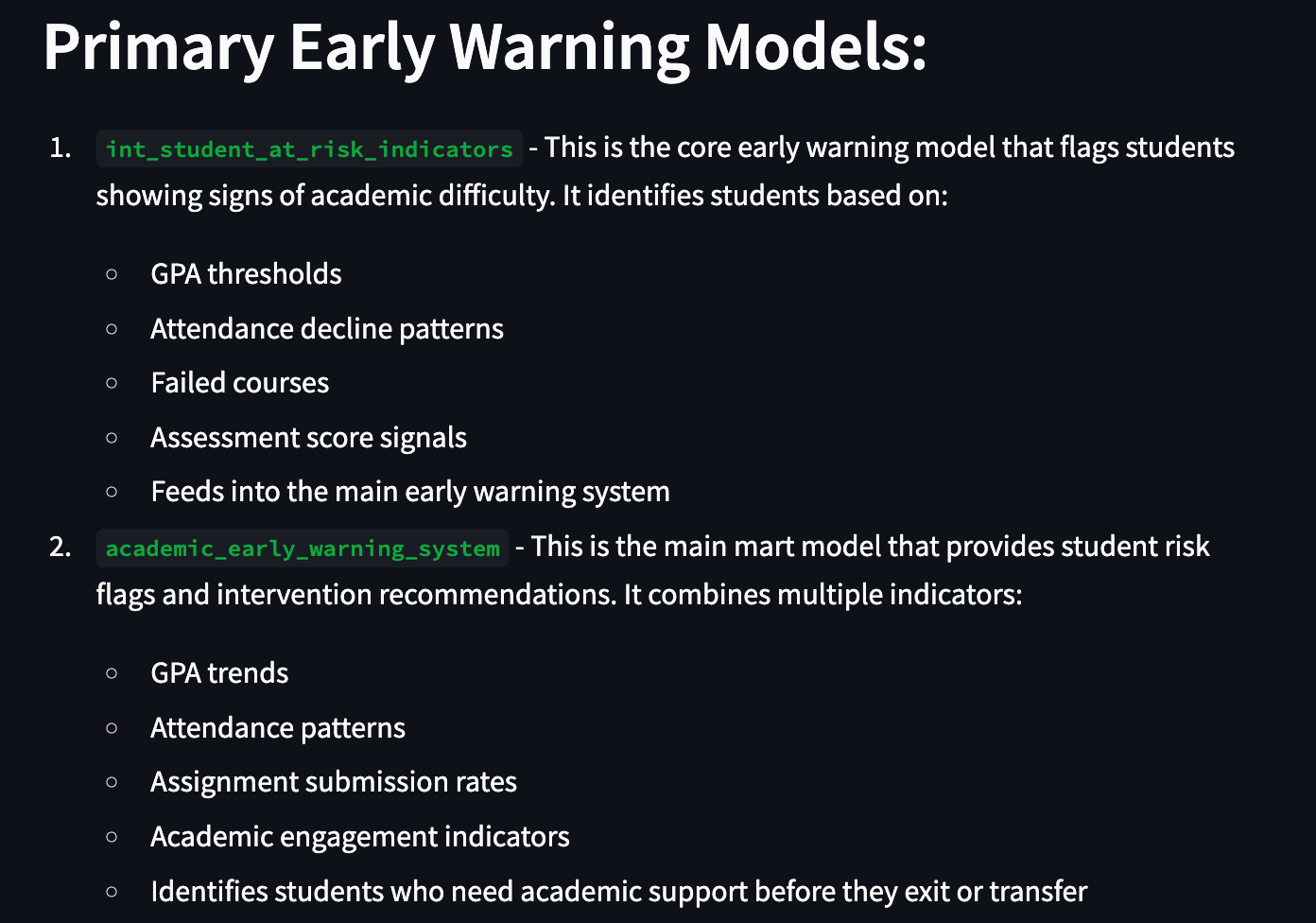
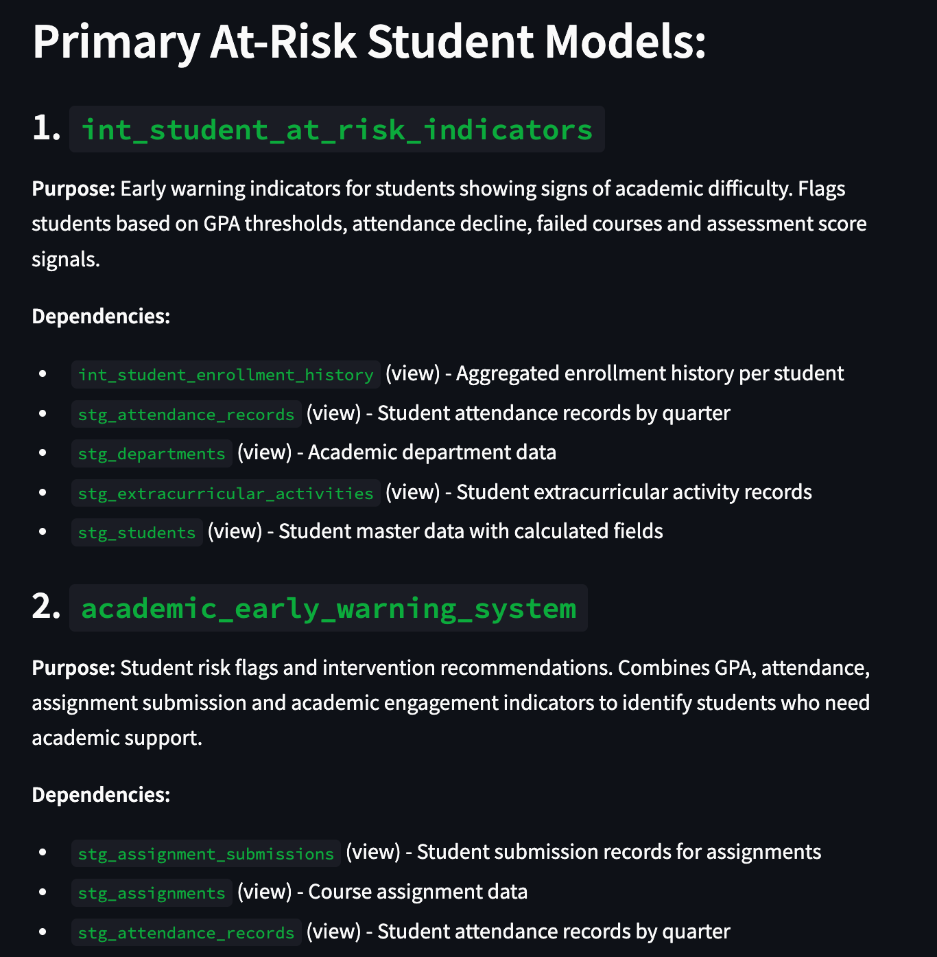
This is the key shift. Questions like “which models track early warning signals for students at academic risk?” or “find me everything related to teacher workload and teaching effectiveness” now work — even if none of the model names contain those words. The graph knows the structure of your project; the embeddings know what it’s about. Together, they cover both.

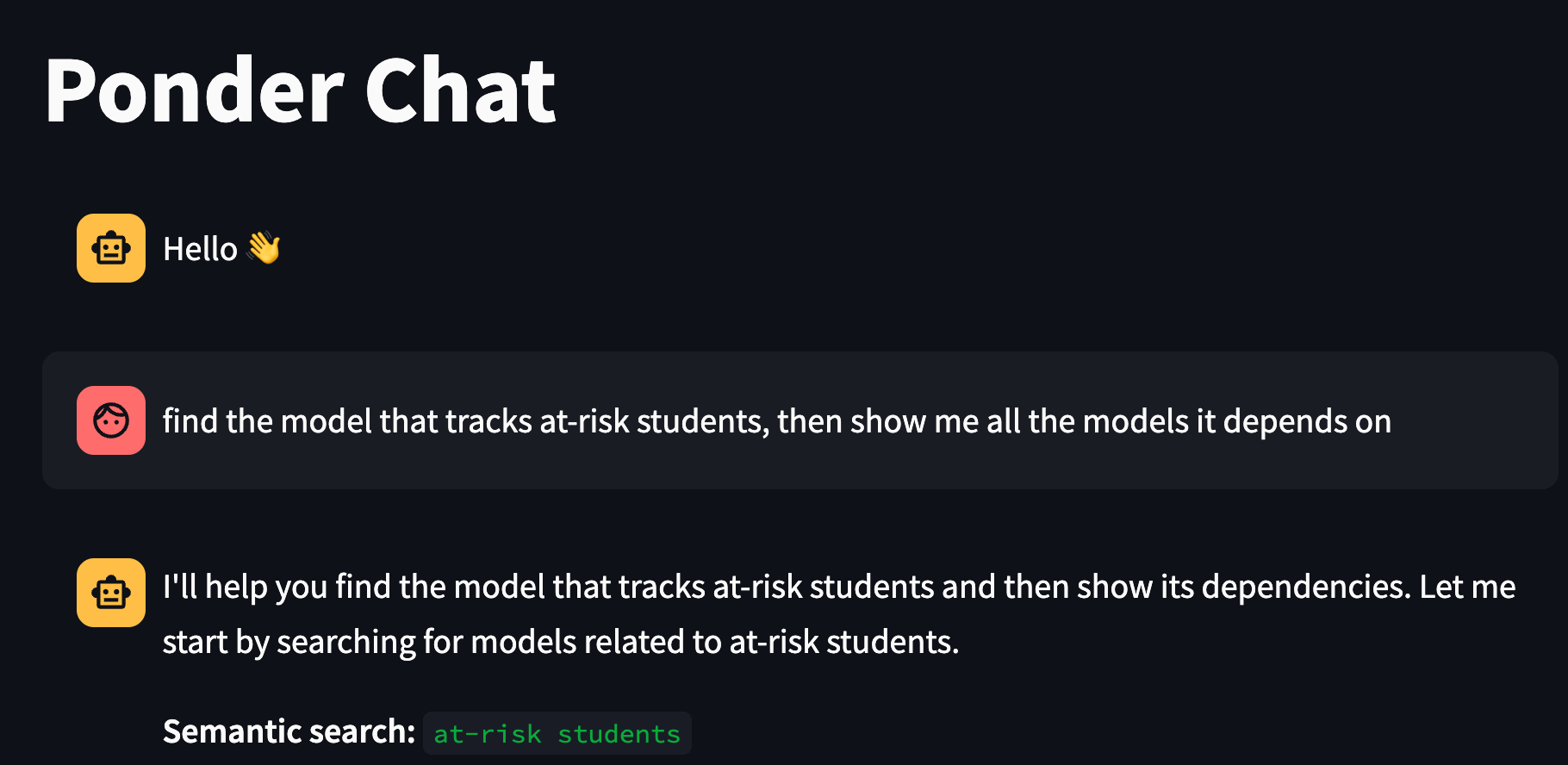
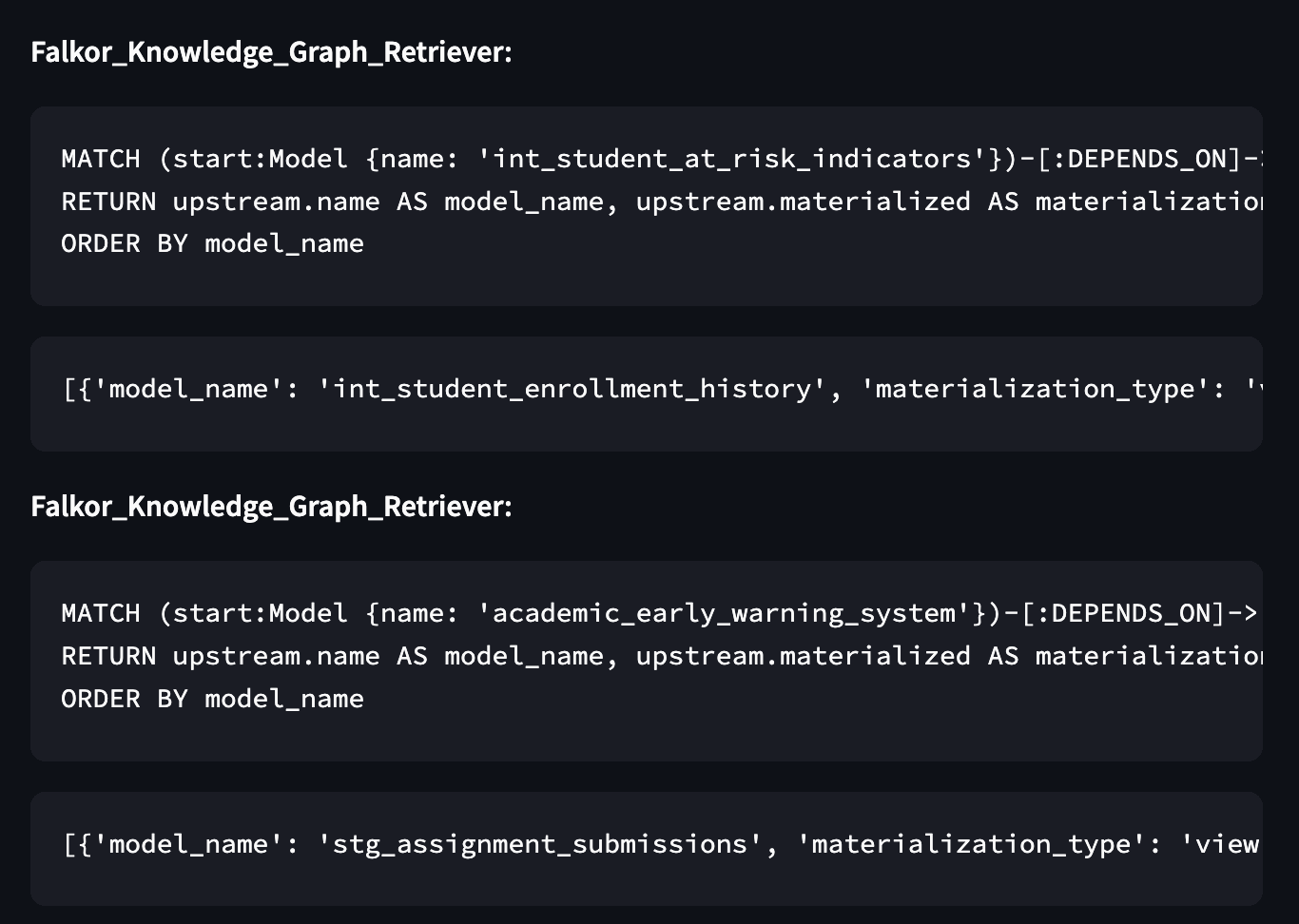
And the two modes compose naturally. You can ask “find the model that tracks at-risk students, then show me all the models it depends on” — the agent uses semantic search to locate the right node, then switches to graph traversal to answer the structural follow-up. That combination is where this really shines.

One honest caveat, though. Traditional RAG pipelines deal with large documents — think long PDFs, sprawling wiki pages, dense technical docs — and a standard best practice there is to chunk them: split each document into smaller pieces, embed each chunk separately, and retrieve only the most relevant chunks at query time. This gives you fine-grained retrieval and avoids stuffing irrelevant content into the LLM’s context.

In our graph setup, we don’t have that luxury in the same way. Each node is a single unit — one model, one embedding. If a node’s combined text (description + all column descriptions) is very long and covers multiple distinct concepts, you can’t retrieve just the relevant part of it; you get the whole node or nothing. You could split a node’s content into multiple embeddings stored as additional attributes, but that quickly becomes unintuitive — you’d be fighting the grain of the graph model rather than working with it. For most dbt projects, where node descriptions are concise and focused, this isn’t a problem in practice. But it’s worth keeping in mind if you’re working with unusually rich metadata or very wide models with dozens of heavily documented columns.

One practical note on embedding providers: the system automatically picks the right model based on your LLM_MODEL_ID prefix — Titan for Bedrock or Anthropic, text-embedding-3-small for OpenAI — so no extra configuration needed.

Full-Text Search

Full-text search has a long history in software engineering. Elasticsearch popularized it at scale, and the core algorithm behind most implementations — BM25 — has been the de facto standard for keyword relevance ranking for decades. The idea is straightforward: score documents by how often the search terms appear in them, adjusted for document length and how rare those terms are across the entire corpus. It’s fast, battle-tested, and remarkably effective when you know what you’re looking for.

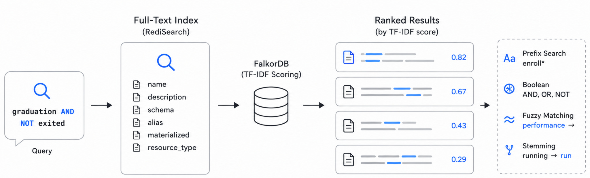
FalkorDB takes a different approach. Its full-text indexing is powered by RediSearch and uses TF-IDF scoring rather than BM25 — similar in spirit, but simpler: it rewards nodes where the search term appears frequently relative to the total number of terms, without BM25’s additional length normalization and term saturation adjustments. For our use case — searching across concise dbt node descriptions rather than long documents — this is a perfectly natural fit. The nodes aren’t essays; the scoring difference between TF-IDF and BM25 rarely matters at this scale.

What does matter is the query expressiveness. And RediSearch delivers. When you upload your manifest, build_fulltext_index() creates a full-text index across six properties on every node — name, description, schema, alias, materialized, and resource_type — for all four label types: Model, Source, Seed, and Snapshot. The FalkorDBFulltextRetriever then queries that index at runtime, deduplicates results across labels, sorts by TF-IDF score, and returns the top matches.

The query syntax is what makes this tool genuinely useful day-to-day:

• Prefix search — enroll* matches “enrollment”, “enrollments”, “enrollee”

• Boolean operators — graduation AND NOT exited, teacher AND workload, risk OR warning

• Fuzzy matching — handles typos via Levenshtein distance, so performence still finds the right models

• Stemming — searching “running” finds “run” and “runs” automatically

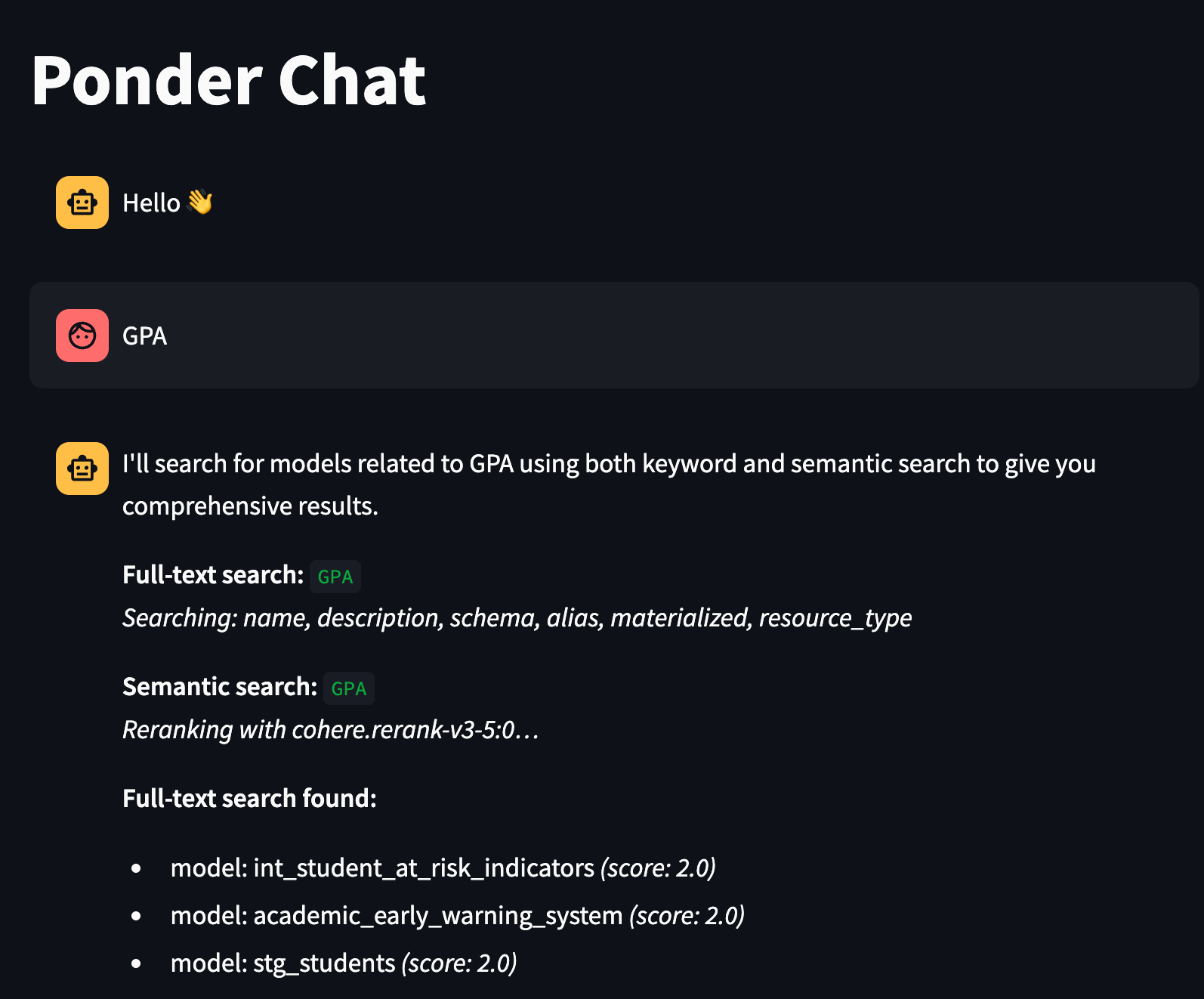
Semantic search is powerful, but it has a blind spot: sometimes you know exactly what you’re looking for. If you need every model that mentions “GPA”, or you want to find anything referencing “attendance” and “retention” together, embedding similarity is overkill — and can actually hurt you by surfacing loosely related models when what you wanted was a precise match.

Full-text search is the right tool for that. The agent knows when to reach for it: use full-text when the question contains specific terms, name fragments, or boolean logic; use semantic search when the question is about a concept or business meaning.

The two tools complement each other cleanly — and as you’ll see next, there’s a third signal we layer on top of semantic search to make sure the most relevant results actually rise to the top.

Reranking

Vector similarity search is good, but it has a subtle problem. When you embed a query and find the closest nodes by cosine distance, you’re measuring how similar two vectors are in a high-dimensional space — and that’s a proxy for relevance, not relevance itself. Embedding models are trained to capture general semantic similarity, not to deeply reason about which result actually best answers a specific question. The result is that KNN search often gets the ballpark right but the ordering wrong. The most relevant node might be ranked 4th or 7th, buried under results that are thematically nearby but not quite what you needed.

This is where reranking comes in.

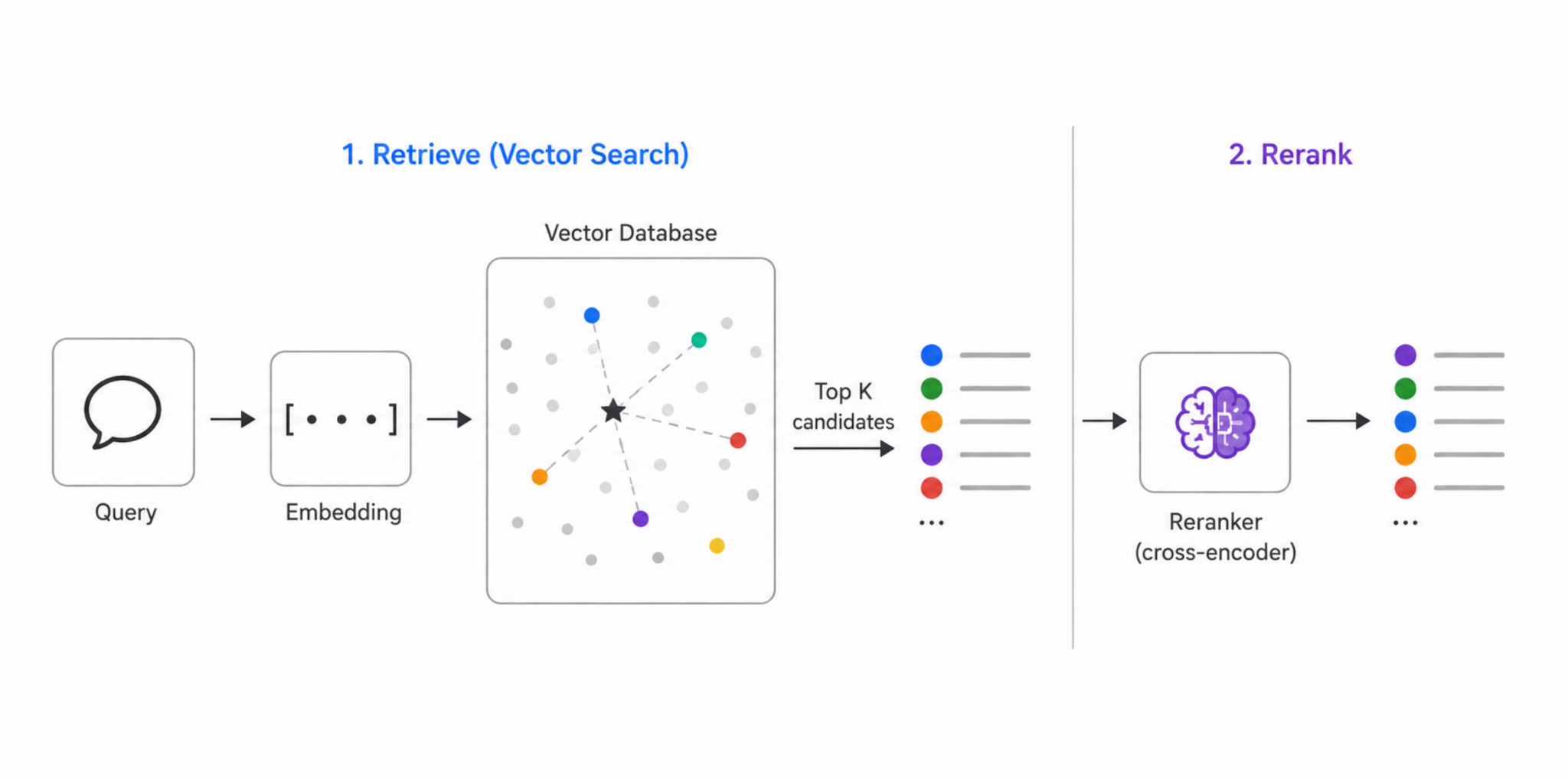
A reranker is a separate model that takes the query and a set of candidate documents — already retrieved by your vector search — and scores each candidate specifically against the query, paying attention to the full meaning of both. Unlike embedding models, which encode the query and each document independently into vectors and then compare them, rerankers look at the query and a candidate together in a single pass. This cross-attention mechanism is much more expensive computationally, which is why you don’t use it to search across your entire dataset — you use it to re-score a small shortlist that vector search already pulled out. The typical pattern is: retrieve 20–50 candidates with KNN, then rerank them and keep the top 5.

We use Amazon Bedrock’s Cohere Rerank v3.5 for this. After FalkorDBNodeRetriever retrieves KNN candidates from FalkorDB, the _rerank() function sends them to Cohere’s reranking model along with the original query, gets back a new relevance ordering, and returns the reranked top results alongside all the original KNN candidates — so you can see exactly what the reranker chose from and why the ordering changed.

To make this tangible, consider a query like “which models track students who are falling behind academically?” Vector search might return 20 candidates that all vaguely relate to students or academics. But the top KNN result by cosine similarity might be a model about GPA trends in general — semantically close to “academic”, but not really about falling behind or at-risk detection. The reranker reads the full query and each candidate together and recognizes that a model specifically described as tracking early warning indicators for academic risk is a much better match — and promotes it accordingly.

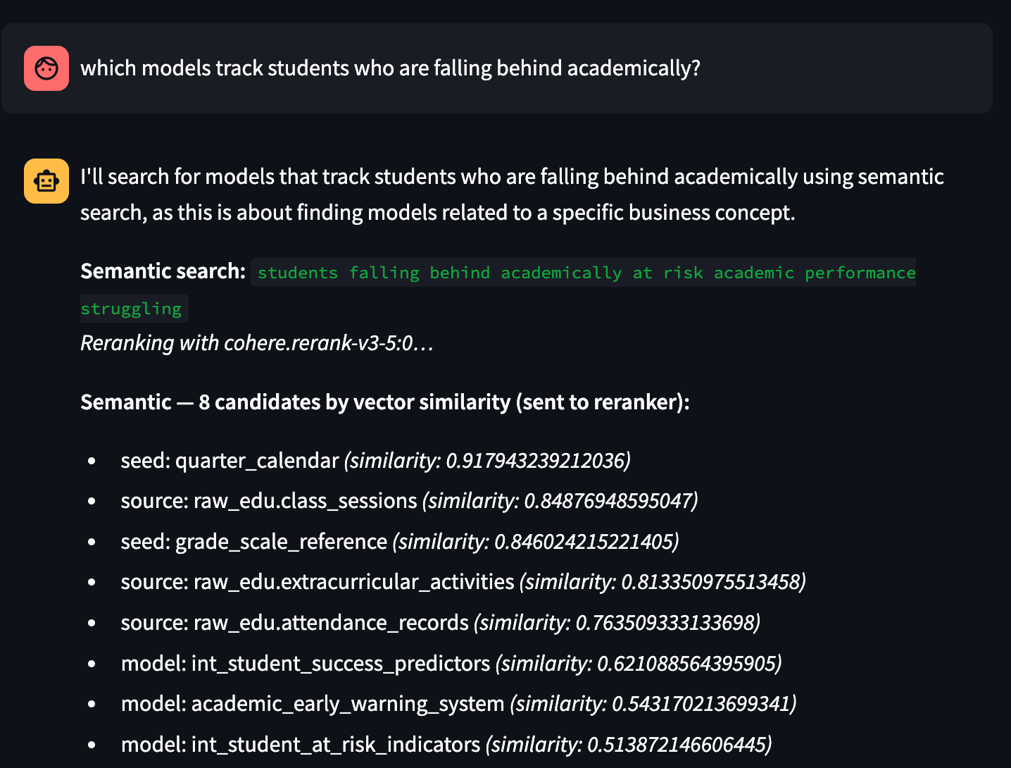
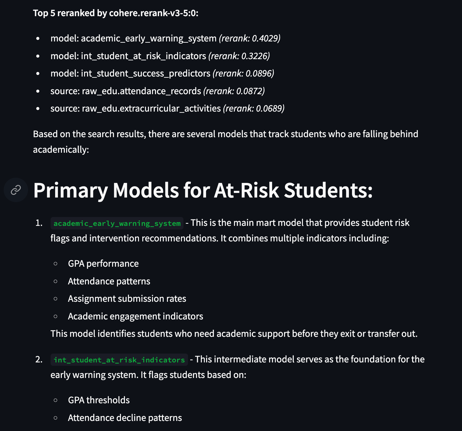
In the Streamlit UI, you can actually watch this happen. We surface both layers: the full set of KNN candidates with their cosine similarity scores, and then the reranked top results with their Cohere relevance scores. Comparing the two orderings is often the most instructive part — you can see precisely where vector similarity and true relevance diverge.

One practical note: reranking only applies to semantic search, not to full-text search. Full-text results are already ranked by TF-IDF term frequency, which is a direct signal of keyword relevance rather than a vector approximation — reranking on top of that would add latency without meaningfully improving precision.

To enable it, just add two environment variables to your .env:

BEDROCK_RERANKER_MODEL_ID=cohere.rerank-v3-5:0
BEDROCK_RERANKER_MODEL_ARN=arn:aws:bedrock:{region}::foundation-model/cohere.rerank-v3-5:0

If Bedrock credentials aren’t configured or the reranker call fails for any reason, the system falls back silently to the original KNN ordering — so it degrades gracefully rather than breaking your pipeline.

Putting It All Together

Let’s zoom out and look at what we’ve built.

The original pipeline gave you a graph. You could traverse it, query it with Cypher, and ask complex structural questions about your dbt project that no other tool could answer. That was already powerful — and judging by the response to the first post, it resonated with a lot of people working on real, complicated dbt projects.

This post added three layers on top of that foundation, and each one fills a gap the previous couldn’t cover:

Graph traversal answers structural questions — lineage, blast radius, dependency chains, test coverage. It speaks the language of relationships. Ask it “what breaks if I drop stg_students?” and it will tell you exactly.

Full-text search answers keyword questions — precise, fast, exact-match retrieval across model names, descriptions, schemas, and more. When you know the term you’re looking for, this is the right tool. Boolean operators, prefix matching, fuzzy tolerance for typos — it handles the cases where you want precision, not approximation.

Semantic search with reranking answers meaning questions — business concepts, vague descriptions, things you can’t quite name but know when you see them. The embeddings live directly on the graph nodes, so there’s no separate vector store to maintain. The reranker then ensures the most genuinely relevant results rise to the top, not just the ones that happen to be closest in vector space.

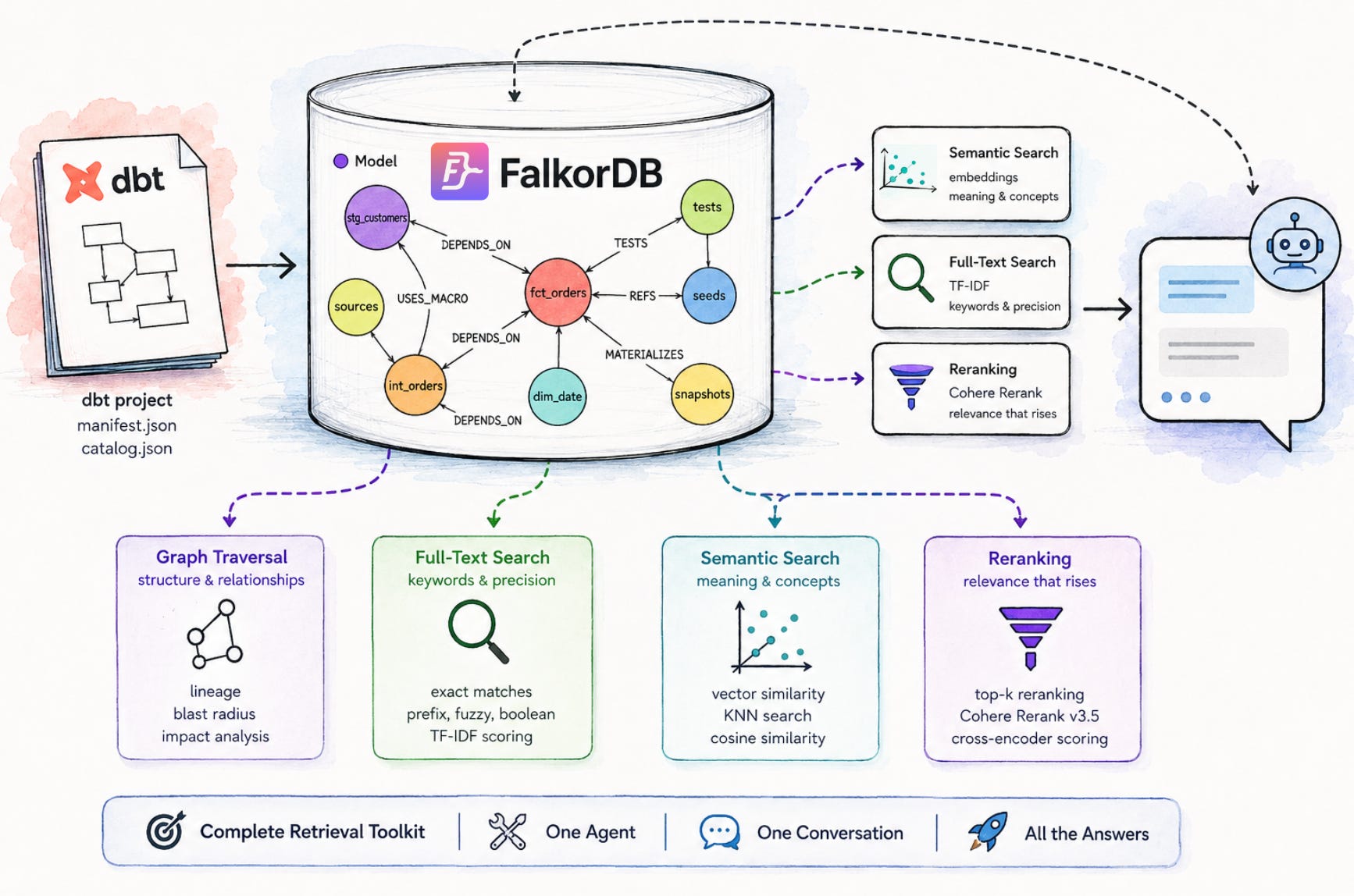
Together, these three tools give the LangGraph agent a complete retrieval toolkit. A question about lineage goes to the graph. A question about a specific term goes to full-text. A question about a concept goes to semantic search, with reranking to sharpen the results. And the most interesting questions — “find the model that tracks at-risk students, then show me everything it depends on” — combine all three in a single conversation turn.

All of this lives in the same dbt-kg repository. Upload your manifest.json and catalog.json, and the pipeline builds the graph, creates the embeddings, and sets up the full-text index automatically. Everything is ready by the time you open the chat.

That said, there are two things we haven’t tackled yet — and they’re worth being honest about. The system understands your dbt project’s structure and metadata deeply, but it doesn’t query your actual data. You can ask which models track student attendance patterns, but you can’t yet ask what the numbers look like right now. And while dbt is the transformation layer, many teams also have a semantic layer sitting on top — tools like dbt Semantic Layer, Cube, or Looker — that define business metrics, dimensions, and how data should be interpreted by end users. Integrating that layer into the same conversational interface would be the natural next step.

So that’s what we’re thinking about next. Stay tuned.